SPSS / PASW Statistics 18 for Mac: The Same Junk as Always

So I write this rant about the horrors of SPSS 16 for Mac. As a result, SPSS Inc. invite me into their beta program for SPSS 17 and offer a free license for it in return. Fair enough. I participate in the program, do all their required testing and submit plenty of bugs. The time window for their beta testers is four weeks. Four weeks. I find that way too short but thats how they operate.

After the end of the beta testing, I never received my free license. I sent them one e-mail about it that was never answered. So when they invited me into their SPSS (which is now called PASW: Predictive Analysis Software) 18 beta, I didn't do anything.

So now PASW 18 ships and I install it with a screen shot app at hand. The first thing I see is this readme window (underlining added by me):
Wow. They still cannot handle foreign characters. I complained about that two versions ago. A company that is producing a statistics software is unable to display a text file containing ä, ö, and ü correctly.

After the install finishes, PASW 18 Mac launches with this gem (you will have to click on it for the large version to see what I mean):

Look at the shadows of "PASW" in the top blue bar and the red line next to it. They are pixelated! These images were obviously produced for a smaller resolution but were magnified to the current size, producing this highly unprofessional experience. So the first two impressions I get give me a feeling that not much care has gone into the production of this software. Attention to detail: Nope, sorry.

The data window features new icons at the top as one can see on the following image.
Unfortunately, that was the only time I ever saw it. After the install, I quit SPSS PASW. Every time I have launched it since them (including after reboots), SPSS PASW crashes on start up:
It. Crashes. On. Every. Launch. On my MacBook Pro (2.33 GHz, 4GB RAM, Mac OS X 10.5.8), SPSS PASW 18 is inoperable. What an enormous piece of junk.

Obtaining the same ANOVA results in R as in SPSS - the difficulties with Type II and Type III sums of squares

I calculated the ANOVA results for my recent experiment with R. In brief, I assumed that women perform poorer in a simulation game (microwolrd) if under stereotype threat than men. My students who assisted in the experiments used SPSS for their calculations. I realized that they obtained different results than I did, with the same model on the same data set. As I was new to R, my initial calculation, an analysis of covariance (ANCOVA) with the dependent variable microworld performance (MWP), the treatment factors gender and stereotype threat, and the covariate reasoning ability, looked like this:

I see two significant main effects of the treatment factors, a significant effect of the covariate, and a significant interaction effect. However, Quick-R tells me this:

WARNING: R provides Type I sequential SS, not the default Type III marginal SS reported by SAS and SPSS. In a nonorthogonal design with more than one term on the right hand side of the equation order will matter (i.e., A+B and B+A will produce different results)! We will need use the drop1( ) function to produce the familiar Type III results.

I do not want order to matter and adjust my calculation accordingly:
What a difference: The main effect of the participants' gender on thir microworld performance does not reach statistical significance. However, that is still not what SPSS produces:

UNIANOVA MWP BY GENDER STTHREAT WITH reasonz
/METHOD=SSTYPE(3)
/INTERCEPT=INCLUDE
/CRITERIA=ALPHA(0.05)
/DESIGN=reasonz GENDER STTHREAT GENDER*STTHREAT.

In SPSS, the main effect of gender is still significant. I dug a little deeper and found another line I needed to add to the R command in order to get exactly the same result:

As you can see, these results are identical. But why all these differences? What does options(contrasts=c("contr.sum", "contr.poly")) actually do and what the heck are Type-III sums of squares? I surely did not learn about these things at my university. I thus did a little reading.

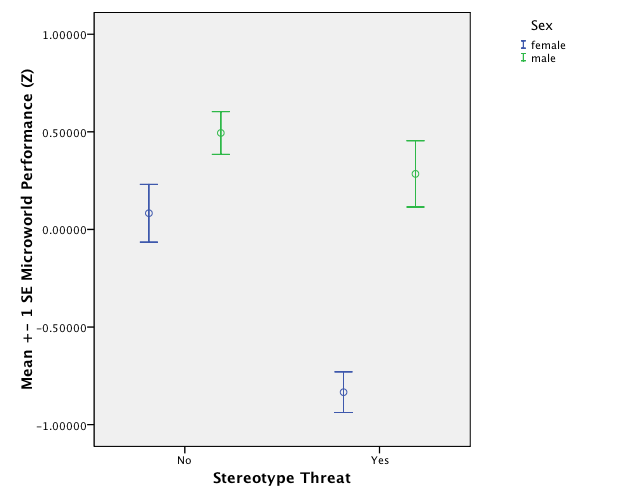
It turns out that the decision about which type of sums of squares to use is based on the question whether it is reasonable to report main effects in the presence of an interaction. Let's review the hypothesis of the experiment: It assumes that women exhibit a decrease in microworld performance under stereotype threat. This is an interaction hypothesis. An error bar plot (lines representing 1 SE) reveals that this is the case:
The plot indicates a significant interaction between gender and stereotype threat. The main effect of stereotype threat is obtained by averaging the performance scores of all participants (both male and female) over the two stereotype threat conditins. This will lead to a low average score under the stereotype threat condition because of the interaction, because the female participants score so extremely low unter stereotype threat and account for the lower average. Thus, it makes no sense to look at the main effect of stereotype threat if an interaction of stereotype threat * gender is present.

Looking for a main effect of stereotype threat under the presence of a significant interaction is a violation of the marginality principle that assumes that all terms to which a particular term is marginal are zero. Lower order terms are marginal to higher order terms, i.e. the main effects of two factors A and B are marginal to the interaction effect A*B. Thus, in this case, the marginality principle would assume that if we inspect and report main effects of gender and stereotype threat, the interaction of stereotype threat and gender is zero. That is not the case and the above example illustrates that - under the given hypothesis - it is useless to report the main effect of stereotype threat.

Now, the problom with Type-III sums of squares (also referred to as marginal sums of squares) is that they are "obtained by fitting each effect after all the other terms in the model, i.e. the Sums of Squares for each effect corrected for the other terms in the model. The marginal (Type III) Sums of Squares do not depend upon the order in which effects are specified in the model" (source). In the case with stereotype threat, that clearly doesn't make any sense: Reporting the Type III sum of squares (as SPSS does per default) for the main effect of stereotype threat means doing so while correcting for the interaction. But it is precisely this interaction that caused the main effect in the first place! Thus, Type-III sums of squares violate the principle of marginality and do not make any sense in the stereotype threat case. Even more so, Type-III sums of squares do "... NOT sum to the Sums of Squares for the model corrected for the mean". I wonder whether this renders the usual way of calculating a factor's effect size eta-square by dividing the SS of the factor by the total SS useless, too?

Anyway, coming back to the ominous contrasts=c("contr.sum", "contr.poly"): In order to obtain the correction for the rest of the factors in the model that Type-III SSs deliver, R needs to know how to balance the factors in the calculation of the SSs. Therefore, it requires a cotrast matrix with zero-sum columns (see here). The R-help for the options() command (?options()) tells us:

contrasts:
the default contrasts used in model fitting such as with aov or lm. A character vector of length two, the first giving the function to be used with unordered factors and the second the function to be used with ordered factors. By default the elements are named c("unordered", "ordered"), but the names are unused.

As the treatment factors gender and stereotype threat are unordered factors, R will use contr.sum in order to construct a contrast matrix of the apropriate order (i.e., 2), because contrasts=c("contr.sum", "contr.poly") was specified. contr.sum(2) produces

[,1]
1 1
2 -1


My first attempt at Type-III SSs in R above produced nonesense and differed from SPSS, because this wasn't specified.Without going into too much detail here (basically because I haven't yet understood everything myself), there is an alternative to the sequence-dependent Type-I SSs and the marginality-violating Type-III SSs: Type II sums of squares preserve the marginality principle. This is how to get them, and this example illustrates that they are diffrent from Type-III SSs and that they are - at least in this case - order independent:
SPSS can do the same by specifying /METHOD=SSTYPE(2) in the UNIANOVA syntax.

The remaining problem in the present case is the main effect of gender. It does make sense to investigate the effect of gender in the presenence of the interaction with stereotype threat, because it could be that women are generally poorer complex problem solvers than men and perform especially poor under stereotype threat on top of the general difference. In fact, the error bar above indicates that this is the case. This leaves me with one main effect that cannot be interpreted (stereotype threat) and another one that can be interpreted. Which SSs should I use? I am a bit lost.

Beautiful Correlation Tables in R

I have achieved another victory in getting R to produce SPSS-like results. In experimental psychology, an analysis of measurement variable correlations is a common method in the course of a statistical analysis. Thus, I wanted R to produce a publication-quality output similar to SPSS: a correlation matrix of measurement variables that contains only the lower triangle of observations, where observations have two decimal digits and are flagged with stars (*, **, and ***) according to levels of statistical significance. However, as statmethods notices:

Unfortunately, neither cor( ) or cov( ) produce tests of significance, although you can use the cor.test( ) function to test a single correlation coefficient.

I did a little research and found this post on the R-help list. I modified Chuck Cleland's code a little so that the following command on the swiss data frame (provided in the Hmisc package) produces a beautiful output:

> corstarsl(swiss[,1:4])

Fertility Agriculture Examination
Fertility
Agriculture 0.35*
Examination -0.65*** -0.69***
Education -0.66*** -0.64*** 0.70***

If one employs the xtable package that produces LaTeX tables from within R, xtable(corstarsl(swiss[,1:4])) produces this:
Isn't that beautiful? I like it a lot. Here's the code (as I said, much of it taken from here):

corstarsl <- function(x){
require(Hmisc)
x <- as.matrix(x)
R <- rcorr(x)$r
p <- rcorr(x)$P

## define notions for significance levels; spacing is important.
mystars <- ifelse(p < .001, "***", ifelse(p < .01, "** ", ifelse(p < .05, "* ", " ")))

## trunctuate the matrix that holds the correlations to two decimal
R <- format(round(cbind(rep(-1.11, ncol(x)), R), 2))[,-1]

## build a new matrix that includes the correlations with their apropriate stars
Rnew <- matrix(paste(R, mystars, sep=""), ncol=ncol(x))
diag(Rnew) <- paste(diag(R), " ", sep="")
rownames(Rnew) <- colnames(x)
colnames(Rnew) <- paste(colnames(x), "", sep="")

## remove upper triangle
Rnew <- as.matrix(Rnew)
Rnew[upper.tri(Rnew, diag = TRUE)] <- ""
Rnew <- as.data.frame(Rnew)

## remove last column and return the matrix (which is now a data frame)
Rnew <- cbind(Rnew[1:length(Rnew)-1])
return(Rnew)
}

More Beautiful Error Bars in R

The rather complex structure and syntax of R (at least to the spoiled SPSS user that I am) comes with a steep learning curve but also with a huge profit: Flexibility. I managed to produce multiple clustered error bars in R today that come across better than a comparable SPSS output:
With regard to my experiment, the graph shows that despite the fact that an ANOVA does not deliver a significant interaction effect of microworld and participant gender, the effect of stereotype threat varies over different microworlds. FSYS produces the smallest gender effects and exhibits the smallest (and statistically insignificant) gender differences in the no stereotype threat condition.

With regard to R, two days of extensive reading and trial-and-error (and my sketchy previous knowledge) have enabled me to achieve almost all the graphical functionality I require (ANOVA interaction plots are next). Maybe R's learning curve isn't that steep after all. What I learned today: the use of the par() function for changing R's graphic output settings and using that to create a multiple figure environment that I then filled with three custom-generated error bars.

Beautiful Error Bars in R

One of the reasons why I haven't made the switch from R to SPSS is R's lack of proper error bar graphs. I use them frequently because they are easy to interpret: If you plot the means of several groups of participants in one error bar chart and scale the error bars to a length of one standard measurement error, non-overlapping error bars indicate a significant difference between the according means. In fact, the APA advocates the use of error bars for reporting results since 2005 [1]. This way of reporting differences in means is also called "Inference by Eye" [1].

After my rants about SPSS, my wise R mentor, Stephan Kolassa, pointed me at the gplots library that features a good function for drawing error bars in R: plotCI(). Stephan also pointed me to Rseek.org, an excellent search engine for R related queries. I fiddled with Stephan's example code in order to reproduce my SPSS clustered error-bar chart from last week's post on stereotype threat in complex problem solving:


And this is how I got in in R:
I like it very much; the only thing I need to work out is how to offset the bars in the same conditions so that overlapping error bars don't actually overlap but are drawn next to each other with a few pixels between them.

If you would like to try this out for yourself, here is the R code that produces the image above:

# Clustered Error Bar for Groups of Cases.
# Example: Experimental Condition (Stereotype Threat Yes/No) x Gender (Male / Female)
# The following values would be calculated from data and are set fixed now for
# code reproduction

means.females <- c(0.08306698, -0.83376319)
stderr.females <- c(0.13655378, 0.06973371)

names(means.females) <- c("No","Yes")
names(stderr.females) <- c("No","Yes")

means.males <- c(0.4942997, 0.2845608)
stderr.males <- c(0.07493673, 0.18479661)

names(means.males) <- c("No","Yes")
names(stderr.males) <- c("No","Yes")

# Error Bar Plot

library (gplots)

# Draw the error bar for female experiment participants:
plotCI(x = means.females, uiw = stderr.females, lty = 2, xaxt ="n", xlim = c(0.5,2.5), ylim = c(-1,1), gap = 0, ylab="Microworld Performance (Z Score)", xlab="Stereotype Threat", main = "Microworld performance over experimental conditions")

# Add the males to the existing plot
plotCI(x = means.males, uiw = stderr.males, lty = 1, xaxt ="n", xlim = c(0.5,2.5), ylim = c(-1,1), gap = 0, add = TRUE)

# Draw the x-axis (omitted above)
axis(side = 1, at = 1:2, labels = names(stderr.males), cex = 0.7)

# Add legend for male and female participants
legend(2,1,legend=c("Male","Female"),lty=1:2)

[1] Cumming, G., & Finch, S. (2005). Inference by Eye: Confidence Intervals and How to Read Pictures of Data. American Psychologist, 60(2), 170–180.

A reply from SPSS Inc.

SPSS Inc. replied to my open letter on the poor quality of SPSS 16 for Mac:

Dear Bertolt:

I want to acknowledge your email/blog and apologize for the inconveniences caused by SPSS 16.0 for Mac. Your bugs, issues and suggestions have been logged and we will work on fixing them in future releases.

We are getting ready to start beta testing SPSS 17.0 for all three platforms -- Windows, Mac and Linux -- in a couple months. Would you like to participate? We would love to have your input. Beta testers get a free copy of the final software.

Thanks,
Arik

________________________
Arik J. Pelkey
Sr. Product Manager
SPSS Inc.
Phone: [deleted]
www.spss.com

________________________________

I do acknowledge the friendly mail and the fact that they didn't try to reason or to justify certain issues. However, note that they apologize for the inconvenience SPSS caused, but not for the bugs, i.e. for the quality of their software. That may sound like splitting hairs, but to me, it's a difference. Why can companies never ever say something like: "We know we screwed up big time. We're sorry." Why does it always have to be some sort of marketing speech? Anyways, I do appreciate their invitation to their beta program which I am going to accept (criticism should always be constructive, eh?).

However, I also suggested two steps on SPSS's part in my reply: Firstly, SPSS should publicly acknowledge certain issues with SPSS 16 for Mac. Secondly, I urge SPSS to review their internal processes for software testing. A more rigorous product testing would have saved them and me a lot of time and nerves.

SPSS 16 for Mac Doesn’t Make the Cut

Mark Kupferberg took up my open letter to SPSS on his Blog. He agrees with me on the poor impression that SPSS 16 for Mac's UI creates:

I haven’t personally seen SPSS 16 for the Mac, but looking at the pictures Bertolt provided, I can certainly see why one might be concerned. It really does look like something that belongs on Windows 3.1.

Some of the people who commented on my rants defended the UI for two main reasons: First, it has been this way since the first release and its good that it stays the same, and second, that it's what Windows users get, too. I think that both views are flawed, because a good piece of software can improve its UI without turning its users away. Changes to the worse have to be avoided of course, but no changes at all just for the sake of stability doesn't sound like a sound argument to me. And secondly no, the Mac UI is not what Windows users are served. The icons on Windows look similar, but they're smaller, integrate better with the overall design and the entire UI makes a more organized impression on me:

Learning R for SAS and SPSS Users

For all of those who as frustrated with SPSS as I am, decisionstats has a great tip:

So you decided to cut down on your Statistical software expenses and decided to get R.

but the problem is you know SAS /SPSS and you need to learn R fast enough to justify switching over …….

the ideal book for you is http://oit.utk.edu/scc/RforSAS&SPSSusers.pdf

SPSS 16 for Mac: Insulting users. An open letter to SPSS Inc.

Dear Ladies and Gentlemen at SPSS Inc,

As a psychologist working in experimental research, the statistical analysis of data is the bread and butter of my daily work. Like the majority of my colleagues in the social sciences, I use the de-facto industry-standard for this task: SPSS; the very product your company is bulit on, the very product that is supposed to deliver a "statistical package for the social sciences" - what SPSS originally stood for before it became a brand.

Let me remind you that this is an exclusive piece of software that comes with a steep price tag of $639 for the single base version for higher-education institutions ($1699 for commercial users).

I am writing you this open letter concerning the quality of your most recent version of SPSS for the Mac - the first version that runs on intel-based Macs, SPSS 16.0 for Mac.

SPSS 16 for Mac - that I have to use on a frequent basis - is the most insulting piece of software I ever came across. I have been frequently annoyed by software in my life time, but this is the first time that I actually feel insulted by a commercial piece of software. Its astonishingly poor interface design and the long list of bugs I discovered during a single week of intense usage make me wonder whether SPSS 16 for Mac was ever used for its intended purpose at your company before you dared to ship it to us - your end users and customers. Do you think that just because we're scientists, you can throw this half-baked crap at us?

The poor impression begins right after double-clicking the icon, when SPSS displays its spalsh screen:

Non-English characters, as they appear in the name of my organization (Universität Zürich), are not displayed correctly. Your programmers have obviously never heard of proper internationalization.

Secondly, the overall appearance makes me think its 1996.

Especially the tool-bar looks exactly like I would expect a toolbar to look like in a 1990s piece of cheap shareware:

I mean, honestly, is this some kind of joke? This interface does neither convey any informational value nor scientific professionalism (if that was intended). The only thing it conveys is your utter lack of interface design principals.

But apart from such minor issues (as you seem to think that UI design is a minor issue), the list of bugs in SPSS that I came across during a single week of working with SPSS 16.0 for Mac is mind-blowing.

• Double-clicking a saved viewer output in the finder opens an empty data file instead. Double-clicking the output in the finder again leads to an error-message that tells me that the file is already open (which it isn't).
• If I go through the cumbersome process of defining input parameters for a data file in text format, and save the parameters as a template for future imports, I cannot load the template the next time I want to use it. When I click on the template file in the open template-dialog, nothing happens.
• If I select "Data... -> Merge Files -> Insert Variables", choose an external file and tell SPSS to add certain variables from that file to my current file while dropping others, the resulting syntax produces an error and nothing happens.
• Importing variables with values that are stored in the decimal format (e. g. "4.023") from a text file produce missing values, i.e. they're not imported at all despite the fact that they're displayed correctly in the preview of the import wizard. Changing the variable type from numeric to string doesn't help.
  
• The menu bar in the output viewer disappears from time to time. Only quitting and restarting SPSS brings it back.
• When re-opening a saved viewer file, the font face of all custom-edited headlines is changed from Arial 16 to Times New Roman 12.
• Overall performance is incredibly slow.
• In the output-viewer, double-clicking a diagram for editing and closing it again sometimes leads to all changes being lost.

These are just the most prominent bugs I came across. I am sure that there is more where that came from. Do you have any kind of testing whatsoever at SPSS? What kind of impression do you think such experiences create? On my part, it creates the impression that you disrespect your users.

According to Eric Sink, there are three categories of software:

• MeWare: The developer creates software. The developer uses it. Nobody else does.
• ThemWare: The developer creates software. Other people use it. The developer does not.
• UsWare: The developer creates software. Other people use it. The developer uses it too.
  

For me, SPSS is an extreme example of ThemWare. You seem to have no clue about the poor quality you're creating - at least for the Mac. This impression is extremely stark because I have to use your products alongside beautifully designed pieces of software such as bibDesk, Apple Pages, and Apple Mail.

In my opinion, there is a piece of statistical software that is just the opposite of SPSS: R. It doesn't sport a graphical interface such as SPSS (it's syntax only, like SPSS used to be), but it's certainly more powerful, creates better graphs, and is built and maintained by a community of people that care for their product and actually use it. I've been trying R alongside SPSS for six months now and I haven't come across a single bug. If R had a powerful graphical interface, your product would be off the market within a week.

My experience with SPSS 16 for Mac will make me change to R once and for all. Furthermore, I will encourage my colleagues to do the same.

Frustrated,
Bertolt Meyer

Note: The link to the three categories of software stems from Jeff Atwoods coding horror.

Update: Two more bugs I can reproduce:

• Copy and Paste from Excel is not working
• Importing Excel Files produces "?" as values after the 40th variable

Update 2: According to this sitemeter-entry, someone from SPSS has read this post. I wonder whether I will receive a reply.

Update 3: The story has been picked up elsewhere and SPSS replied.