The Swiss Ban on Minarets Confirms the Contact Hypothesis

In November 2009, Switzerland held a referendum that sought approval for a constitutional ban on minarets. 57.5% of the voters supported the ban. The ban was supported by the Swiss right wing party SVP. Poster ads that supported the ban used images as the ones below, tapping on anti-muslim sentiments and on diffuse fear towards muslims. Thus, the referendum has been widely interpreted as a vote against foreigners by the media.

A student of mine, Michael Jäckli, had the idea to use archival polling data from the referendum for a test of Alport's Contact Hypothesis. It suggests that "interpersonal contact is one of the most effective ways to reduce prejudice between majority and minority group members". Thus, Swiss municipalities (the smallest unit for which polling data is available from the Swiss bureau of statistics) with a low percentage of foreign nationals should show a high rate of approval of the ban, while municipalities with a high percentage of foreigners should show a lower rate of approval.

In order to test this assumption, Michael obtained the agreement to the ban on the municipal level from the Swiss bureau of statistics, along with indicators for educational level and social-economic status for the municipalities. He was then able to regress the agreement for the ban on the percentage of foreigners:

As visible in the plot, municipalities with a below-average percentage of foreigners tended to accept the ban at above-average levels. Without controlling for other variables, an increase of the percentage of foreigners in a municipality by 1% would decrease its agreement to the ban by 0.37%.

As lower education and social status is usually associated with more right-wing political views, Michael tested whether the negative relationship between the percentage of foreigners and the approval of the ban still holds under statistical control of these two variables. The according stepwise hierarchical regression is presented below.

It reveals that low economic status and low educational levels are indeed associated with an acceptance of the ban. But even if these factors are controlled for, there is still a significant yet small negative effect of the percentage of foreigners on the approval of the ban: Municipalities with a low percentage of foreigners tended to support the ban.

Why does an increase of the percentage of foreigners decrease the support for the ban on minarets? Possibly because municipalities can profit from their foreign population: An inspection of the bivariate correlations of the measurement variables (see below) reveals that the percentage of foreigners is associated with higher levels of education and social-economic status.

The R code that produced these results can be found below. Michael's data set can be downloaded in .CSV-Format here.

# import the data

minarettdata <- read.csv(file = "minarettdata.csv")

# inspect the data

head(minarettdata)

length(minarettdata$municipality_nr)

# make the data available

attach(minarettdata)

# generate the plot

plot(foreigners, minarett_approval, main = "Approval of the minaret ban in all Swiss municipalities\nas a function of municipal share of foreign nationals", xlab = "Municipal share of foreign nationals (in %)", ylab = "Municipal share of voters approving the ban (in %)")

abline(lm(minarett_approval ~ foreigners), col = "blue")

abline(h = 57.5, lty = 2)

abline(v = 22, lty = 2)

text(x = 60, y= 48, round(coef(lm(minarett_approval ~ foreigners))[2], digits = 2), col = "blue")

text(x = 22, y = 26, "Swiss-wide share of foreign nationals (22%)", cex = .70, pos = 4)

text(x = 49, y = 60, "Swiss-wide approval of the\nban on minarets (57.5%)", cex = .70, pos = 4)

mean(foreigners)

mean(minarett_approval)

# test the stepwise regression

library(QuantPsyc)

lmodel.1 <- lm(minarett_approval ~ SES + edu_level)

summary(lmodel.1)

lm.beta(lmodel.1)

lmodel.2 <- lm(minarett_approval ~ SES + edu_level + foreigners)

summary(lmodel.2)

lm.beta(lmodel.2)

# determine the significance of the increase in R-squared

anova(lmodel.1, lmodel.2)

# print the correlation table

corstarsl2(minarettdata[,2:5])

library(xtable)

xtable(print(corstarsl2(minarettdata[,2:5])))

# clean up

rm(minarettdata, lmodel.1, lmodel.2)

An R Function for the Blau Index of Diversity

In diversity research, one is often interested in how an individual feature is distributed among the members of a group. In other words, one is interested in how diverse a group is with regard to that feature. If the particular feature can be expressed in a metric way, e.g. age or organizational tenure, researchers use measures of dispersion for quantifying the diversity of a group with regard to that feature. For example, the standard deviation of the average age of group members can be employed to indicate the age diversity of a group.

If researchers wish to quantify the diversity of a group with regard to a nominal feature, such as ethnicity, gender, or education, they usually employ the Blau Index (Blau, 1977). The Blau Index is calculated by
where p is the proportion of group members in a given category and i is the number of different categories of the feature across all groups. If a group is homogeneous with regard to the feature in question, i.e., if all group members have the same nationality, the Blau Index of the group for nationality is 0. If all members of the group have a different nationality, the Blau Index of that group for nationality approaches 1. The maximum Blau Index for a feature in a given data set depends on the number of categories of that feature in the data set.

A number of studies have linked the Blau Index of (management-) teams to team processes and team outcomes (e.g., Bantel & Jackson, 1989; Richard, Barnett, Dwyer, & Chadwick, 2004; Chandler, Honig, & Wiklund, 2005; Pitts, 2005). Threfore, I also wanted to include the Blau Index for various features in the analysis of the data I obtained in an attempt to replicate and extend a study by Homan, van Knippenberg, van Kleef, & De Dreu (2007).

In doing so, I was unable to locate an R function for calculating the Blau Index. I therefore wrote my own and thought that others might also find it useful.

The function takes two arguments:
A numeric vector, groupID, denoting the group of every person/participant in the data set.
A second vector, feat, that can be either numeric or string, denoting the expression of the feature for each person/participant in the data set.

The function returns a vector of length = number of groups with the Blau Index for each group.

Example:

groupid <- c(1,1,1,2,2,2,2)
feature <- c("male", "male", "male", "female", "female", "male", "male")

blau.index(groupid, feature)

[1] 0.0 0.5

Here is the code:

blau.index <- function(groupid, feat){
blau.index <- rep(0, length(levels(as.factor(groupid))))
if (is.numeric(feat)) { # if the feature is denoted as a numeric ordinal variable
for (i in 1:length(levels(as.factor(groupid)))){
for (j in 1:length(levels(as.factor(feat)))){
blau.index[i] <- blau.index[i] + ((sum(feat[groupid == i & feat == j])/j)/ length(feat[groupid == i]))^2
}
}
} else { # if the feature is denoted as as strings
number.of.features <- length(levels(as.factor(feat)))
feat.num <- rep(NA, times = length(as.factor(feat)))
for (i in 1:number.of.features){
feat.num[feat == levels(as.factor(feat))[i]] <- i
feat.num[is.na(feat.num)] <- (number.of.features + 1)
}
for (i in 1:length(levels(as.factor(groupid)))){
for (j in 1:length(levels(as.factor(feat.num)))){
blau.index[i] <- blau.index[i] + ((sum(feat.num[groupid == i & feat.num == j])/j)/ length(feat.num[groupid == i]))^2
}
}
}
blau.index <- (1 - blau.index)
return(blau.index)
}

I would appreciate suggestions for improvements.

References

Blau, P. M. (1977). Inequality and heterogeneity. New York, NY: Free Press.

Bantel, K., & Jackson, S. (1989). Top management and innovations in banking: does the composition of the top team make a difference? Strategic Management Journal, 10, 107–124.

Chandler, G. N., Honig, B., & Wiklund, J. (2005). Antecedents, moderators, and performance consequences of membership change in new venture teams. Journal of Business Venturing, 20, 705–725.

Homan, A. C., van Knippenberg, D., Kleef, G. A. van, & De Dreu, C. K. W. (2007). Bridging faultlines by valuing diversity: Diversity beliefs, information elaboration, and performance in diverse work groups. Journal of Applied Psychology, 92(5), 1189–1199.

Pitts, D. (2005). Diversity, representation, and performance: Evidence about race and ethnicity in public organizations. Journal of Public Administration Research and Theory, 15, 615–631.

Richard, O., Barnett, T., Dwyer, S., & Chadwick, K. (2004). Cultural diversity in management, firm performance, and the moderating role of entrepreneurial orientation dimensions. Academy of Management Journal, 47, 255–266.

Obtaining the same ANOVA results in R as in SPSS - the difficulties with Type II and Type III sums of squares

I calculated the ANOVA results for my recent experiment with R. In brief, I assumed that women perform poorer in a simulation game (microwolrd) if under stereotype threat than men. My students who assisted in the experiments used SPSS for their calculations. I realized that they obtained different results than I did, with the same model on the same data set. As I was new to R, my initial calculation, an analysis of covariance (ANCOVA) with the dependent variable microworld performance (MWP), the treatment factors gender and stereotype threat, and the covariate reasoning ability, looked like this:

I see two significant main effects of the treatment factors, a significant effect of the covariate, and a significant interaction effect. However, Quick-R tells me this:

WARNING: R provides Type I sequential SS, not the default Type III marginal SS reported by SAS and SPSS. In a nonorthogonal design with more than one term on the right hand side of the equation order will matter (i.e., A+B and B+A will produce different results)! We will need use the drop1( ) function to produce the familiar Type III results.

I do not want order to matter and adjust my calculation accordingly:
What a difference: The main effect of the participants' gender on thir microworld performance does not reach statistical significance. However, that is still not what SPSS produces:

UNIANOVA MWP BY GENDER STTHREAT WITH reasonz
/METHOD=SSTYPE(3)
/INTERCEPT=INCLUDE
/CRITERIA=ALPHA(0.05)
/DESIGN=reasonz GENDER STTHREAT GENDER*STTHREAT.

In SPSS, the main effect of gender is still significant. I dug a little deeper and found another line I needed to add to the R command in order to get exactly the same result:

As you can see, these results are identical. But why all these differences? What does options(contrasts=c("contr.sum", "contr.poly")) actually do and what the heck are Type-III sums of squares? I surely did not learn about these things at my university. I thus did a little reading.

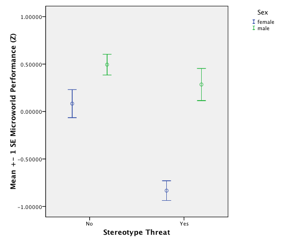
It turns out that the decision about which type of sums of squares to use is based on the question whether it is reasonable to report main effects in the presence of an interaction. Let's review the hypothesis of the experiment: It assumes that women exhibit a decrease in microworld performance under stereotype threat. This is an interaction hypothesis. An error bar plot (lines representing 1 SE) reveals that this is the case:
The plot indicates a significant interaction between gender and stereotype threat. The main effect of stereotype threat is obtained by averaging the performance scores of all participants (both male and female) over the two stereotype threat conditins. This will lead to a low average score under the stereotype threat condition because of the interaction, because the female participants score so extremely low unter stereotype threat and account for the lower average. Thus, it makes no sense to look at the main effect of stereotype threat if an interaction of stereotype threat * gender is present.

Looking for a main effect of stereotype threat under the presence of a significant interaction is a violation of the marginality principle that assumes that all terms to which a particular term is marginal are zero. Lower order terms are marginal to higher order terms, i.e. the main effects of two factors A and B are marginal to the interaction effect A*B. Thus, in this case, the marginality principle would assume that if we inspect and report main effects of gender and stereotype threat, the interaction of stereotype threat and gender is zero. That is not the case and the above example illustrates that - under the given hypothesis - it is useless to report the main effect of stereotype threat.

Now, the problom with Type-III sums of squares (also referred to as marginal sums of squares) is that they are "obtained by fitting each effect after all the other terms in the model, i.e. the Sums of Squares for each effect corrected for the other terms in the model. The marginal (Type III) Sums of Squares do not depend upon the order in which effects are specified in the model" (source). In the case with stereotype threat, that clearly doesn't make any sense: Reporting the Type III sum of squares (as SPSS does per default) for the main effect of stereotype threat means doing so while correcting for the interaction. But it is precisely this interaction that caused the main effect in the first place! Thus, Type-III sums of squares violate the principle of marginality and do not make any sense in the stereotype threat case. Even more so, Type-III sums of squares do "... NOT sum to the Sums of Squares for the model corrected for the mean". I wonder whether this renders the usual way of calculating a factor's effect size eta-square by dividing the SS of the factor by the total SS useless, too?

Anyway, coming back to the ominous contrasts=c("contr.sum", "contr.poly"): In order to obtain the correction for the rest of the factors in the model that Type-III SSs deliver, R needs to know how to balance the factors in the calculation of the SSs. Therefore, it requires a cotrast matrix with zero-sum columns (see here). The R-help for the options() command (?options()) tells us:

contrasts:
the default contrasts used in model fitting such as with aov or lm. A character vector of length two, the first giving the function to be used with unordered factors and the second the function to be used with ordered factors. By default the elements are named c("unordered", "ordered"), but the names are unused.

As the treatment factors gender and stereotype threat are unordered factors, R will use contr.sum in order to construct a contrast matrix of the apropriate order (i.e., 2), because contrasts=c("contr.sum", "contr.poly") was specified. contr.sum(2) produces

[,1]
1 1
2 -1


My first attempt at Type-III SSs in R above produced nonesense and differed from SPSS, because this wasn't specified.Without going into too much detail here (basically because I haven't yet understood everything myself), there is an alternative to the sequence-dependent Type-I SSs and the marginality-violating Type-III SSs: Type II sums of squares preserve the marginality principle. This is how to get them, and this example illustrates that they are diffrent from Type-III SSs and that they are - at least in this case - order independent:
SPSS can do the same by specifying /METHOD=SSTYPE(2) in the UNIANOVA syntax.

The remaining problem in the present case is the main effect of gender. It does make sense to investigate the effect of gender in the presenence of the interaction with stereotype threat, because it could be that women are generally poorer complex problem solvers than men and perform especially poor under stereotype threat on top of the general difference. In fact, the error bar above indicates that this is the case. This leaves me with one main effect that cannot be interpreted (stereotype threat) and another one that can be interpreted. Which SSs should I use? I am a bit lost.

Beautiful Correlation Tables in R

I have achieved another victory in getting R to produce SPSS-like results. In experimental psychology, an analysis of measurement variable correlations is a common method in the course of a statistical analysis. Thus, I wanted R to produce a publication-quality output similar to SPSS: a correlation matrix of measurement variables that contains only the lower triangle of observations, where observations have two decimal digits and are flagged with stars (*, **, and ***) according to levels of statistical significance. However, as statmethods notices:

Unfortunately, neither cor( ) or cov( ) produce tests of significance, although you can use the cor.test( ) function to test a single correlation coefficient.

I did a little research and found this post on the R-help list. I modified Chuck Cleland's code a little so that the following command on the swiss data frame (provided in the Hmisc package) produces a beautiful output:

> corstarsl(swiss[,1:4])

Fertility Agriculture Examination
Fertility
Agriculture 0.35*
Examination -0.65*** -0.69***
Education -0.66*** -0.64*** 0.70***

If one employs the xtable package that produces LaTeX tables from within R, xtable(corstarsl(swiss[,1:4])) produces this:
Isn't that beautiful? I like it a lot. Here's the code (as I said, much of it taken from here):

corstarsl <- function(x){
require(Hmisc)
x <- as.matrix(x)
R <- rcorr(x)$r
p <- rcorr(x)$P

## define notions for significance levels; spacing is important.
mystars <- ifelse(p < .001, "***", ifelse(p < .01, "** ", ifelse(p < .05, "* ", " ")))

## trunctuate the matrix that holds the correlations to two decimal
R <- format(round(cbind(rep(-1.11, ncol(x)), R), 2))[,-1]

## build a new matrix that includes the correlations with their apropriate stars
Rnew <- matrix(paste(R, mystars, sep=""), ncol=ncol(x))
diag(Rnew) <- paste(diag(R), " ", sep="")
rownames(Rnew) <- colnames(x)
colnames(Rnew) <- paste(colnames(x), "", sep="")

## remove upper triangle
Rnew <- as.matrix(Rnew)
Rnew[upper.tri(Rnew, diag = TRUE)] <- ""
Rnew <- as.data.frame(Rnew)

## remove last column and return the matrix (which is now a data frame)
Rnew <- cbind(Rnew[1:length(Rnew)-1])
return(Rnew)
}

More Beautiful Error Bars in R

The rather complex structure and syntax of R (at least to the spoiled SPSS user that I am) comes with a steep learning curve but also with a huge profit: Flexibility. I managed to produce multiple clustered error bars in R today that come across better than a comparable SPSS output:
With regard to my experiment, the graph shows that despite the fact that an ANOVA does not deliver a significant interaction effect of microworld and participant gender, the effect of stereotype threat varies over different microworlds. FSYS produces the smallest gender effects and exhibits the smallest (and statistically insignificant) gender differences in the no stereotype threat condition.

With regard to R, two days of extensive reading and trial-and-error (and my sketchy previous knowledge) have enabled me to achieve almost all the graphical functionality I require (ANOVA interaction plots are next). Maybe R's learning curve isn't that steep after all. What I learned today: the use of the par() function for changing R's graphic output settings and using that to create a multiple figure environment that I then filled with three custom-generated error bars.

Beautiful Error Bars in R

One of the reasons why I haven't made the switch from R to SPSS is R's lack of proper error bar graphs. I use them frequently because they are easy to interpret: If you plot the means of several groups of participants in one error bar chart and scale the error bars to a length of one standard measurement error, non-overlapping error bars indicate a significant difference between the according means. In fact, the APA advocates the use of error bars for reporting results since 2005 [1]. This way of reporting differences in means is also called "Inference by Eye" [1].

After my rants about SPSS, my wise R mentor, Stephan Kolassa, pointed me at the gplots library that features a good function for drawing error bars in R: plotCI(). Stephan also pointed me to Rseek.org, an excellent search engine for R related queries. I fiddled with Stephan's example code in order to reproduce my SPSS clustered error-bar chart from last week's post on stereotype threat in complex problem solving:


And this is how I got in in R:
I like it very much; the only thing I need to work out is how to offset the bars in the same conditions so that overlapping error bars don't actually overlap but are drawn next to each other with a few pixels between them.

If you would like to try this out for yourself, here is the R code that produces the image above:

# Clustered Error Bar for Groups of Cases.
# Example: Experimental Condition (Stereotype Threat Yes/No) x Gender (Male / Female)
# The following values would be calculated from data and are set fixed now for
# code reproduction

means.females <- c(0.08306698, -0.83376319)
stderr.females <- c(0.13655378, 0.06973371)

names(means.females) <- c("No","Yes")
names(stderr.females) <- c("No","Yes")

means.males <- c(0.4942997, 0.2845608)
stderr.males <- c(0.07493673, 0.18479661)

names(means.males) <- c("No","Yes")
names(stderr.males) <- c("No","Yes")

# Error Bar Plot

library (gplots)

# Draw the error bar for female experiment participants:
plotCI(x = means.females, uiw = stderr.females, lty = 2, xaxt ="n", xlim = c(0.5,2.5), ylim = c(-1,1), gap = 0, ylab="Microworld Performance (Z Score)", xlab="Stereotype Threat", main = "Microworld performance over experimental conditions")

# Add the males to the existing plot
plotCI(x = means.males, uiw = stderr.males, lty = 1, xaxt ="n", xlim = c(0.5,2.5), ylim = c(-1,1), gap = 0, add = TRUE)

# Draw the x-axis (omitted above)
axis(side = 1, at = 1:2, labels = names(stderr.males), cex = 0.7)

# Add legend for male and female participants
legend(2,1,legend=c("Male","Female"),lty=1:2)

[1] Cumming, G., & Finch, S. (2005). Inference by Eye: Confidence Intervals and How to Read Pictures of Data. American Psychologist, 60(2), 170–180.

Learning R for SAS and SPSS Users

For all of those who as frustrated with SPSS as I am, decisionstats has a great tip:

So you decided to cut down on your Statistical software expenses and decided to get R.

but the problem is you know SAS /SPSS and you need to learn R fast enough to justify switching over …….

the ideal book for you is http://oit.utk.edu/scc/RforSAS&SPSSusers.pdf